Global Redistributions

In high performance computing large multidimensional arrays are often distributed and shared amongst a large number of different processors. Consider a large three-dimensional array of double (64 bit) precision and global shape \((512, 1024, 2048)\). To lift this array into RAM requires 8 GB of memory, which may be too large for a single, non-distributed machine. If, however, you have access to a distributed architecture, you can split the array up and share it between, e.g., four CPUs (most supercomputers have either 2 or 4 GB of memory per CPU), which will only need to hold 2 GBs of the global array each. Moreover, many algorithms with varying degrees of locality can take advantage of the distributed nature of the array to compute local array pieces concurrently, effectively exploiting multiple processor resources.

There are several ways of distributing a large multidimensional array. Two such distributions for our three-dimensional global array (using 4 processors) are shown below

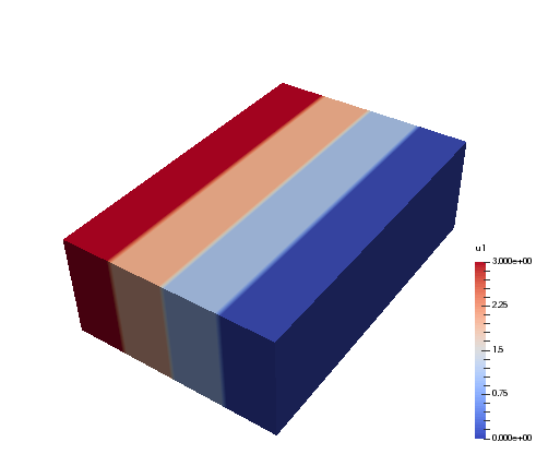
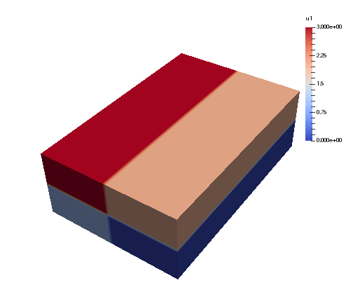
Here each color represents one of the processors. We note that in the first image only one of the three axes is distributed, whereas in the second two axes are distributed. The first configuration corresponds to a slab, whereas the second corresponds to a pencil distribution. With either distribution only one quarter of the large, global array needs to be kept in rapid (RAM) memory for each processor, which is great. However, some operations may then require data that is not available locally in its quarter of the total array. If that is so, the processors will need to communicate with each other and send the necessary data where it is needed. There are many such MPI routines designed for sending and receiving data.

We are generally interested in algorithms, like the FFT, that work on the global array, along one axis at the time. To be able to execute such algorithms, we need to make sure that the local arrays have access to all of its data along this axis. For the figure above, the slab distribution gives each processor data that is fully available along two axes, whereas the pencil distribution only has data fully available along one axis. Rearranging data, such that it becomes aligned in a different direction, is usually termed a global redistribution, or a global transpose operation. Note that with mpi4py-fft we always require that at least one axis of a multidimensional array remains aligned (non-distributed).

Distribution and global redistribution is in mpi4py-fft handled by three classes in the pencil module:

• Pencil

• Subcomm

• Transfer

These classes are the low-level backbone of the higher-level PFFT and DistArray classes. To use these low-level classes directly is not recommended and usually not necessary. However, for clarity we start by describing how these low-level classes work together.

Lets first consider a 2D dataarray of global shape (8, 8) that will be distributed along axis 0. With a high level API we could then simply do:

import numpy as np
from mpi4py_fft import DistArray
N = (8, 8)
a = DistArray(N, [0, 1])

where the [0, 1] list decides that the first axis can be distributed, whereas the second axis is using one processor only and as such is aligned (non-distributed). We may now inspect the low-level Pencil class associated with a:

p0 = a.pencil

The p0 Pencil object contains information about the distribution of a 2D dataarray of global shape (8, 8). The distributed array a has been created using the information that is in p0, and p0 is used by a to look up information about the global array, for example:

>>> a.alignment
1
>>> a.global_shape
(8, 8)
>>> a.subcomm
(<mpi4py.MPI.Cartcomm at 0x10cc14a68>, <mpi4py.MPI.Cartcomm at 0x10e028690>)
>>> a.commsizes
[1, 1]

Naturally, the sizes of the communicators will depend on the number of processors used to run the program. If we used 4, then a.commsizes would return [1, 4].

We note that a low-level approach to creating such a distributed array would be:

import numpy as np
from mpi4py_fft.pencil import Pencil, Subcomm
from mpi4py import MPI
comm = MPI.COMM_WORLD
N = (8, 8)
subcomm = Subcomm(comm, [0, 1])
p0 = Pencil(subcomm, N, axis=1)
a0 = np.zeros(p0.subshape)

Note that this last array a0 would be equivalent to a, but it would be a pure Numpy array (created on each processor) and it would not contain any of the information about the global array that it is part of (global_shape, pencil, subcomm, etc.). It contains the same amount of data as a though and a0 is as such a perfectly fine distributed array. Used together with p0 it contains exactly the same information as a.

Since at least one axis needs to be aligned (non-distributed), a 2D array can only be distributed with one processor group. If we wanted to distribute the second axis instead of the first, then we would have done:

a = DistArray(N, [1, 0])

With the low-level approach we would have had to use axis=0 in the creation of p0, as well as [1, 0] in the creation of subcomm. Another way to get the second pencil, that is aligned with axis 0, is to create it from p0:

p1 = p0.pencil(0)

Now the p1 object will represent a (8, 8) global array distributed in the second axis.

Lets create a complete script (pencils.py) that fills the array a with the value of each processors rank (note that it would also work to follow the low-level approach and use a0):

import numpy as np
from mpi4py_fft import DistArray
from mpi4py import MPI
comm = MPI.COMM_WORLD
N = (8, 8)
a = DistArray(N, [0, 1])
a[:] = comm.Get_rank()
print(a.shape)

We can run it with:

mpirun -np 4 python pencils.py

and obtain the printed results from the last line (print(a.shape)):

(2, 8)
(2, 8)
(2, 8)
(2, 8)

The shape of the local a arrays is (2, 8) on all 4 processors. Now assume that we need these data aligned in the x-direction (axis=0) instead. For this to happen we need to perform a global redistribution. The easiest approach is then to execute the following:

b = a.redistribute(0)
print(b.shape)

which would print the following:

(8, 2)
(8, 2)
(8, 2)
(8, 2)

Under the hood the global redistribution is executed with the help of the Transfer class, that is designed to transfer data between any two sets of pencils, like those represented by p0 and p1. With low-level API a transfer object may be created using the pencils and the datatype of the array that is to be sent:

transfer = p0.transfer(p1, np.float)

Executing the global redistribution is then simply a matter of:

a1 = np.zeros(p1.subshape)
transfer.forward(a, a1)

Now it is important to realise that the global array does not change. The local a1 arrays will now contain the same data as a, only aligned differently. However, the exchange is not performed in-place. The new array is as such a copy of the original that is aligned differently. Some images, Fig. 1 and Fig. 2, can be used to illustrate:

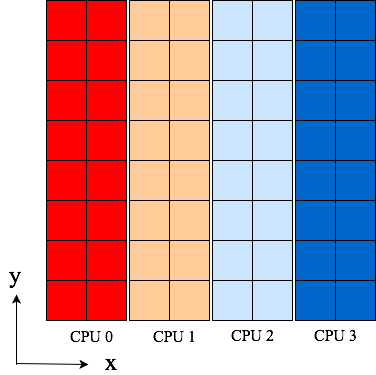
Fig. 1 Original 4 pencils (p0) of shape (2, 8) aligned in y-direction. Color represents rank.

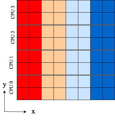
Fig. 2 4 pencils (p1) of shape (8, 2) aligned in x-direction after receiving data from p0. Data is the same as in Fig. 1, only aligned differently.

Mathematically, we will denote the entries of a two-dimensional global array as \(u_{j_0, j_1}\), where \(j_0\in \textbf{j}_0=[0, 1, \ldots, N_0-1]\) and \(j_1\in \textbf{j}_1=[0, 1, \ldots, N_1-1]\). The shape of the array is then \((N_0, N_1)\). A global array \(u_{j_0, j_1}\) distributed in the first axis (as shown in Fig. 1) by processor group \(P\), containing \(|P|\) processors, is denoted as

\[u_{j_0/P, j_1}\]

The global redistribution, from alignment in axis 1 to alignment in axis 0, as from Fig. 1 to Fig. 2 above, is denoted as

\[u_{j_0, j_1/P} \xleftarrow[P]{1\rightarrow 0} u_{j_0/P, j_1}\]

This operation corresponds exactly to the forward transfer defined above:

transfer.forward(a0, a1)

If we need to go the other way

\[u_{j_0/P, j_1} \xleftarrow[P]{0\rightarrow 1} u_{j_0, j_1/P}\]

this corresponds to:

transfer.backward(a1, a0)

Note that the directions (forward/backward) here depends on how the transfer object is created. Under the hood all transfers are executing calls to MPI.Alltoallw.

Multidimensional distributed arrays

The procedure discussed above remains the same for any type of array, of any dimensionality. With mpi4py-fft we can distribute any array of arbitrary dimensionality using any number of processor groups. We only require that the number of processor groups is at least one less than the number of dimensions, since one axis must remain aligned. Apart from this the distribution is completely configurable through the classes in the pencil module.

We denote a global \(d\)-dimensional array as \(u_{j_0, j_1, \ldots, j_{d-1}}\), where \(j_m\in\textbf{j}_m\) for \(m=[0, 1, \ldots, d-1]\). A \(d\)-dimensional array distributed with only one processor group in the first axis is denoted as \(u_{j_0/P, j_1, \ldots, j_{d-1}}\). If using more than one processor group, the groups are indexed, like \(P_0, P_1\) etc.

Lets illustrate using a 4-dimensional array with 3 processor groups. Let the array be aligned only in axis 3 first (\(u_{j_0/P_0, j_1/P_1, j_2/P_2, j_3}\)), and then redistribute for alignment along axes 2, 1 and finally 0. Mathematically, we will now be executing the three following global redistributions:

(1)\[\begin{split}u_{j_0/P_0, j_1/P_1, j_2, j_3/P_2} \xleftarrow[P_2]{3 \rightarrow 2} u_{j_0/P_0, j_1/P_1, j_2/P_2, j_3} \\ u_{j_0/P_0, j_1, j_2/P_1, j_3/P_2} \xleftarrow[P_1]{2 \rightarrow 1} u_{j_0/P_0, j_1/P_1, j_2, j_3/P_2} \\ u_{j_0, j_1/P_0, j_2/P_1, j_3/P_2} \xleftarrow[P_0]{1 \rightarrow 0} u_{j_0/P_0, j_1, j_2/P_1, j_3/P_2}\end{split}\]

Note that in the first step it is only processor group \(P_2\) that is active in the redistribution, and the output (left hand side) is now aligned in axis 2. This can be seen since there is no processor group there to share the \(j_2\) index. In the second step processor group \(P_1\) is the active one, and in the final step \(P_0\).

Now, it is not necessary to use three processor groups just because we have a four-dimensional array. We could just as well have been using 2 or 1. The advantage of using more groups is that you can then use more processors in total. Assuming \(N = N_0 = N_1 = N_2 = N_3\), you can use a maximum of \(N^p\) processors, where \(p\) is the number of processor groups. So for an array of shape \((8,8,8,8)\) it is possible to use 8, 64 and 512 number of processors for 1, 2 and 3 processor groups, respectively. On the other hand, if you can get away with it, or if you do not have access to a great number of processors, then fewer groups are usually found to be faster for the same number of processors in total.

We can implement the global redistribution using the high-level DistArray class:

N = (8, 8, 8, 8)
a3 = DistArray(N, [0, 0, 0, 1])
a2 = a3.redistribute(2)
a1 = a2.redistribute(1)
a0 = a1.redistribute(0)

Note that the three redistribution steps correspond exactly to the three steps in (1).

Using a low-level API the same can be achieved with a little more elaborate coding. We start by creating pencils for the 4 different alignments:

subcomm = Subcomm(comm, [0, 0, 0, 1])
p3 = Pencil(subcomm, N, axis=3)
p2 = p3.pencil(2)
p1 = p2.pencil(1)
p0 = p1.pencil(0)

Here we have defined 4 different pencil groups, p0, p1, p2, p3, aligned in axis 0, 1, 2 and 3, respectively. Transfer objects for arrays of type np.float are then created as:

transfer32 = p3.transfer(p2, np.float)
transfer21 = p2.transfer(p1, np.float)
transfer10 = p1.transfer(p0, np.float)

Note that we can create transfer objects between any two pencils, not just neighbouring axes. We may now perform three different global redistributions as:

a0 = np.zeros(p0.subshape)
a1 = np.zeros(p1.subshape)
a2 = np.zeros(p2.subshape)
a3 = np.zeros(p3.subshape)
a0[:] = np.random.random(a0.shape)
transfer32.forward(a3, a2)
transfer21.forward(a2, a1)
transfer10.forward(a1, a0)

Storing this code under pencils4d.py, we can use 8 processors that will give us 3 processor groups with 2 processors in each group:

mpirun -np 8 python pencils4d.py

Note that with the low-level approach we can now easily go back using the reverse backward method of the Transfer objects:

transfer10.backward(a0, a1)

A different approach is also possible with the high-level API:

a0.redistribute(out=a1)
a1.redistribute(out=a2)
a2.redistribute(out=a3)

which corresponds to the backward transfers. However, with the high-level API the transfer objects are created (and deleted on exit) during the call to redistribute and as such this latter approach may be slightly less efficient.